How Does a Bike-Share Navigate Speedy Success?

• Preamble
• Scenario
• Data Acquisition and Cleaning
  • Raw Data Download
  • Data Cleaning
• Data Analysis
  • Ride Durations and Types
  • Biking to Work
  • Seasonal Behaviour
• Odds & Ends
• Key Insights

Preamble

This project is one of the suggested capstone projects that conclude the Google Data Analytics Certificate.

All data in this project was warehoused in a local Microsoft SQL Server installation. Data transformation and analysis was carried out using KNIME Analytics Platform, a powerful and extensible open-source software for graphical data analysis and data science. Visualizations were created using Tableau Public.

Scenario

In this scenario, we find ourselves employed with a fictional bike-sharing company in Chicago that offers thousands of available bikes across hundreds of docking stations throughout the city.¹ Customers can unlock and ride the bikes between these stations by buying either single-ride or single-day passes (classifying them as “casual” customers) or becoming subscribed members through an annual fee.

The director of marketing believes that the best way forward for the company is to focus on converting casual customers into subscribed members. To this end, we are tasked with analyzing how these two different customer types differ in their use of the bike-sharing service, and identifying strategies to most effectively approach casual customers and advertise an upgrade to a membership.

Data Acquisition and Cleaning

Raw Data Download

To conduct our analysis, we use one year’s worth of data describing the rides that both casual and subscribed customers have made with the company’s biked. The data is taken from the publicly available download page of Divvy (accessed June 8, 2021) and covers a time frame from the beginning of April 2020 to the end of April 2021.

Within the downloaded zip archives, we find csv files ranging from ca. 10 to 110 megabyte in size. The files contain the following information about each ride made with company bikes:

• ride_id: a unique identifier for each record;
• rideable_type: the type of bicycle used;
• started_at and ended_at: the start and end date- and time stamps;
• start_station_name, start_station_id, and their end_ equivalents: names and identifiers for the start and end stations;
• start_lat, start_lon, and their end_ equivalents: the latitude and longitude of the start and end stations, in decimal degrees; and
• member_casual: the customer type that carried out the trip.

For the given time frame, a total of 3,826,978 records are recovered from the raw data files.

Given the large number of records, it is infeasible to approach the data set using spreadsheet software such as Microsoft Excel. Instead, let us first upload the data from all csv files into a single “raw” SQL table, _RideData_Raw. At this stage, we store all fields as varchar types without assigning a primary key.

After unpacking all csv files into a dedicated folder (and setting them to write-only access to avoid inadvertent modification), we construct a KNIME workflow that loops over all of these files and inserts their data into the SQL table.

The KNIME workflow used for full raw data upload

Data Cleaning

Missing Values. After dumping all available raw data into the monolithic _RideData_Raw table, we go on to investigate what kind of mess we’re dealing with. A quick glance at the data reveals that there are quite a number of NULLs in the ..._station_name and ..._station_id fields. In all, there are 273,273 records with at least one of the relevant fields nulled, which is equal to about 7% of the full data set. Not great, not terrible. We’ll come back to them later.

Ride Durations and Duplicates. The ride_id values might be useful to use as primary keys for the data, but we must first assure that they are indeed unique. Unfortunately, there are 209 duplicate values (each appearing twice), which we copy into a _RideData_Raw_Duplicates table for further analysis.

Upon closer inspection, we each one of these duplicate values appears in pairs of two—one with its end date before the start date. Obviously, this is faulty data. Luckily, the other entry each has a valid end date after the start date, so that we can simply discard these faulty records and use their meaningful siblings.

As a little reward on the side, we find that all raw data records with invalid ride dates (end before start) are caught by these duplicates. That’s one less thing to worry about.

Data Normalization. It is immediately obvious that there is a lot of redundant information in the original data: Each row carries both a ..._station_id and a ..._station_name field, together with latitude and longitude information, for both the start and end stations. Obviously, we can eliminate these redundancies if we only store the unique station identifiers with each record, offloading the additional information into a lookup table.

The bad news however is that there are 1,267 distinct station IDs, but only 714 station names in the raw data after ignoring all NULLs. In other words, a lot of the stations have more than one id assigned to them. We could create new unique identifiers for the stations and put a bridge table between the raw data and the lookup table. For the sake of simplicity however, we will simply forget about the station IDs at this point and use only the station names to identify them.

Station Names and Locations. Ultimately, a docking station is characterized by its physical location, while its name is only derived from nearby streets and landmarks. Thus, the most important piece of information that we have about the stations are the latitude and longitude values in the original data. As we look at the _lat and _lng values for some sample stations however, we notice that their values also jitter to some extent.² To figure out the station locations, we need to apply some form of averaging to these coordinates. Some of the raw data, however, comes with only four decimal figures (which corresponds to a resolution of about 11 m) or even fewer—the worst offenders even have none at all (equivalent to 111 km of resolution). To judge the accuracy of the averaged locations, we thus include the standard deviation of the station coordinates. The overall data is saved in a Stations table, with station_name as the primary key.³

During the process of this data cleaning, we also notice that some of the station names seem to be duplicated with either a (*) or (Temp) suffix—such as Smith Park (*) and Wood St & Taylor St (Temp). The latter appears to indicate stations that were temporarily relocated, while the meaning of the former is unclear. The starred stations do, however, not significantly differ from their “parent” stations without the suffix. For simplicity, we choose to simply drop the (*) suffixes when evaluating station names, while retaining the (Temp) ones.⁴

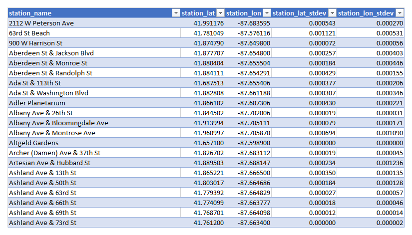
Excerpt of the station location data

Main Ride Data. After we have decided to offload the station location information into a separate table and eliminated duplicates and NULLs, we can transfer the raw data into a new table, RideData, with the following fields:

• ride_id (primary key);
• bike_type (copied from rideable_type in the raw data);
• start_day, start_time and their end_ equivalents (split into day and time fields from the raw data);
• ride_duration (the time difference in minutes between the start and end times);
• start_station and end_station (the station names as used in the Stations table); and
• customer_type (copy of member_casual from the raw data).

At this point, we have a data set of 3,553,496 valid and unique ride records. Unfortunately, the data does not allow us to identify how many subscribed members the company actually has, and how many of the casual customers are returning ones; so we won’t be able to make detailed statements about the customer base, only about the ride data. In addition, the values of the bike_type data are not quite clear. The entries electric_bike and classic_bike seem to be obvious enough, but a larger number of records has a rather obscure value of docked_bike. Since the data comes without further explanation, we will ignore the bike_type data for now; in a real-world setting, we would have to inquire about the meaning of these categories.

Data Analysis

Ride Durations and Types

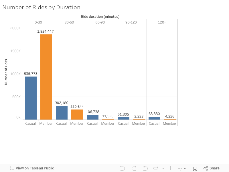
To start out with our analysis, we sort all ride durations into 30-minute bins and investigate their frequency. The results already paint a very interesting picture: The vast majority (about 78%) of all recorded trips are less than 30 minutes long, and members make twice as many of these trips as casual customers. Conversely, trips of more than 30 minutes are taken more often by casual customers than by members. This of course begs the question: Why do subscribed members prefer shorter trips by such a big margin? As the next section below will show, there might be a very compelling explanation for this behaviour.

When investigating customer behaviour, another interesting question comes to mind: Do people generally return bikes to the same stations where they started their trips, or do they drop them off at a different one? Let’s call the first type a “round trip” and the second one an “one-way trip.” By grouping all rides in the data into one of these categories, we find the following picture:

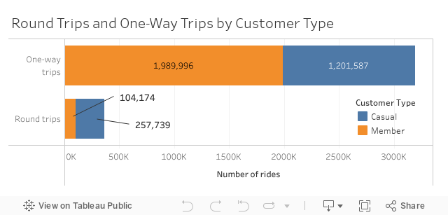
Clearly, round trips are far more prevalent than one-way trips across both customer types. If someone does a round trip, however, they are more likely to be a casual customer.

Biking to Work

In the introductory notes to the project, we are given the interesting piece of information that about 30% of customers use the company’s biked to cycle to work. In order to dig deeper into this behaviour of our riders, let’s take a look at the spatial and temporal distribution of rides both during workdays and weekends.

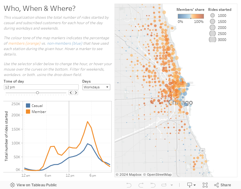
During weekends, casual and subscribed customers do not show much of a difference in their ride behaviour. On workdays, however, the difference is striking! Members significantly outperform casual customers in the number of rides, with two very distinct spikes around 7 am and 5 pm. This seems to corroborate what was mentioned to us about “Biking to work”; we can see that this is much more popular with members than with casual customers. This might explain the different behaviours in the ride duration data we saw above.

From the spatial distribution of rides on the map and the size of the markers for each station, we can also tell that most of them are started around the Downtown area of Chicago. While that may not be all that surprising, the colour coding of the markers is far more interesting, indicating the balance of members vs. casual customers starting their rides at each station. Those stations with a higher patronage of casual customers than members (blue hues) again tend to aggregate on the eastern edge of the city along the coastline and around the Downtown area, whereas the western, inland parts are dominated by subscribed members. In other words: This map tells us where to find the casual customers to which we want to advertise our subscription model.

Seasonal Behaviour

Let’s now group the number of rides by months to investigate how ridership behaviour changes across the seasons.

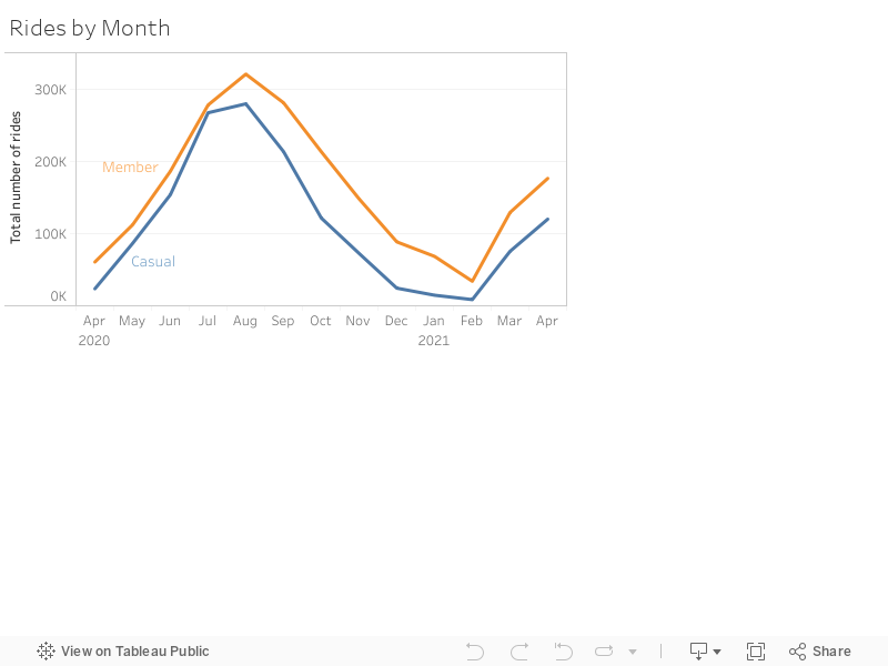
Not much of a surprise here: The bikes see most of their use during the summer months, more so by members than casual customers; and the gap between the two customer segments gets more pronounced during the winter months.⁵ An interesting thing to note however is the rather abrupt uptick in ride numbers in March 2021, and the drastically increased numbers in April 2021 compared to the previous year. Immediately, the increasing Covid-19 vaccination rate and the (at least perceived) end of the pandemic come to mind; it is reasonable to assume that more people were willing to be out and about, and returning to work, around this time.

Odds & Ends

More for fun than productive analysis, let’s have look at the duration (in minutes) and the distances of all one-way trips (calculated from the station locations) of all rides in the data set. Both quantities are described well by a log-normal distribution (red lines).⁶

Counts of ride durations and distances (left) and 25-hour anomaly (right)

There are some notable quirks in the ride duration data. One is a sudden spike in ride numbers around the 1500-minute (25-hour) mark; presumably, this is an artifact introduced by the algorithms that track the ride durations by capping some rides after a certain amount of time. The other anomaly are a number of records that extend to very long ride durations, with 269 rides being longer than 10,000 minutes (ca. one week), and 20 rides being longer than one 40,000 minutes (ca. one month.)

Key Insights

Based on the above analysis, we can report the following findings to the marketing team:

Casual customers…

… make an overall slightly smaller amount of rides than subscribed members, at a ca. 3:4 ratio.

… are more likely than subscribed members to make longer trips of more than 30 minutes duration.

… are more likely to start trips around the “touristy” downtown and coastline areas of the city.

… are more likely than subscribed members to make (rather unpopular) round trips.

Subscribed members…

… are much more likely than casual customers to use the bikes to travel to and from work on workdays.

… greatly dominate the number of short rides of less than 30 minutes.

… start more rides in the inland portion of the city.

… are more likely than casual customers to make one-way trips.

Both customer types…

… strongly prefer one-way trips to round trips.

… show about the same preference for ride hours during the weekends.

… unsurprisingly prefer to bike in the summer months rather than winter.

Overall, this information should help the marketing team to find the right time and locations to more effectively advertise membership upgrades to casual customers.