Fake News and Dirty Data

• Preamble
• The Dataset
  • Data Quality
  • Data Cleaning
• Processing and Model Building
  • What is “Fake News”, Really?
  • Lemmatization and Stop Words
  • Feature Selection
• Modeling
  • Single Decision Tree
  • Random Forest
  • Logistic Regression

Preamble

Among the many datasets available on kaggle.com is one called “Fake and real news”, with its description spelling out a challenge: “Can you use this data set to make an algorithm able to determine if an article is fake news or not ?”

Let’s see if we can!

Please note that Natural Language Processing is very much a field in its own right, and one that I am making contact with for the first time here; things are necessarilry going to be rather rough around the edges in terms of textual analysis. The main idea behind this article is to explore the data preparation and conditioning for machine learning models.

The Dataset

The dataset contains two csv files with news articles classified as either “fake” or “true”, each file holding more than 20,000 records. We find the following fields in the files:

• title: the title of the published article;
• text: the full text of the article;
• subject: a subject categorization of the article;
• date: the publication date of the article (2016 and 2017).

More explanations on the collection methodology and the various fields are available in an external PDF file: ¹

This dataset was collected from real-world sources; the truthful articles were obtained by crawling articles from Reuters.com (News website). As for the fake news articles, they were collected from different sources. The fake news articles were collected from unreliable websites that were flagged by Politifact (a fact-checking organization in the USA) and Wikipedia. The dataset contains different types of articles on different topics, however, the majority of articles focus on political and World news topics.
The dataset consists of two CSV files. The first file named “True.csv” contains more than 12,600 articles from reuter.com. The second file named “Fake.csv” contains more than 12,600 articles from different fake news outlet resources. (…) The data collected were cleaned and processed, however, the punctuations and mistakes that existed in the fake news were kept in the text.

Data Quality

A good data analysis will start with the source and quality of the data itself, so let’s take a close look at the dataset and its accompanying PDF notes. At the risk of being overly nitpicky, here are some peculiarities that stand out:

1. All “true” news stem from a single source (Reuters), which poses the danger of introducing a lot of bias into this part of the dataset. The authors don’t explain why no other news agencies, like AP or DPA, were included.
2. The “fake” news articles are sourced from a more diverse background, but unfortunately we get no detailed information about those sources. A high-quality dataset would include the original article URLs as well.
3. The source for the “true” news articles is misspelt in the explanatory PDF notes. “reuter.com” leads to the website of a German retailer for bathroom products. The website of the Reuters news agency is “reuters.com”. This is not a huge problem in itself, but still gives off an unpleasant impression of sloppy work.
4. For some reason, the notes also point out that each category contains “more than 12,600 articles” of “fake” and “true” news each. That’s technically correct,² but also an example of being “oddly specific”. (Perhaps these notes were typed out for an earlier version of the dataset and not updated later on when more articles were added?)
5. The notes state that the data was cleaned, but do not explain how.
6. As for the subject field, all Reuters articles are labeled either “politicsNews” or “worldnews”. The labels on the “fake” articles are somewhat more granular, but only mildly more helpful: “Government News”, “US_News”, “left-news”, “News” and “politics”. We get no information how these labels were assigned, and more crucially, why there are no common labels between the “true” and “fake” data sets.

Overall, the subject field doesn’t really give us anything useful to work with, so we’ll just ignore it from now on. Likewise, we’ll leave the publication dates aside and focus on the article titles and bodies for our analysis.

Data Cleaning

Despite the claims in the PDF notes that the data was cleaned, there are also a number of “junk” entries that we need to deal with: Rows that only contain URLs, duplicate entries, missing text bodies, etc. A cursory look at the data also reveals another problem. All of the articles in the “true” data subset start with a preamble like “WASHINGTON (Reuters)”. Including these text fragments later on would cause feature leakage, and our model would simply learn to pick out this preamble to judge whether an article is fake news.³ Similarly, a lot of the entries in the “fake” data include image source attributions that look like “Featured image via…” which causes the same problem. Thus, we need to strip these parts from the valid entries as well.

All data cleaning is done in Python, using the pandas and re regex packages.⁴

To remove the “leaky” bits of data mentioned before, we would ideally have some way to detect the according parts in the articles automatically. Otherwise, we will have to manually craft a detection and removal strategy for each piece of harmful “meta”-information separately. For simplicity, we will choose the latter approach here and run each article through a series of regular expression (regex) matches in order to remove the problematic text fragments. At the same time, we can take some other steps to improve the quality of the text data: Removing any non-printable characters like tabs and newlines; eliminating non-text artifacts such as URLs, embedded JavaScript code, etc.; and correcting parsing errors where words and punctuation are not properly separated by whitespaces.

First, all rows with duplicated article titles and bodies are filtered out; this eliminates 5573 entries (!) from the “fake” and 220 entries from the “true” data.⁵ Then, rows with invalid entries (empty title or text fields, containing URLs, …) are removed; this eliminates a further 508 “fake” and only a single “true” article. Finally, we find that there are 95 entries in the “true” data that are simply uncommented tweets from Trump’s official twitter account, and since they contain no other reporting, we remove these as well.

In the end, we are left with 17400 “fake” and 21101 “true” articles.

Processing and Model Building

Before we dive deeper into analyzing and transforming the data, we have to ask ourselves: What exactly do we want to model with this data? Or, in more practical terms: What will be the inputs and outputs to our models?

What is “Fake News”, Really?

Obviously, we want to build some sort of classifier that tells us whether a given article is likely to be fake news or not. That, in turn, raises the issue of how we define “fake news” in the first place. Since we are using a pre-supplied dataset, we are constrained by the contents of that data; in this regard, fake news could be most concisely be characterized as sensationalis, emotionally loaded and heavily editorialized content. The subject of the reporting itself may give an indication as to how likely a piece of writing is to be fake news, but is not necessarily a hard criterion; you can do both factual and sensationalized reporting on the same subject. Likewise, the publication date of an article does not give much of an indication either.

Consequently, metadata alone won’t suffice to categorize articles as “fake” or “true”. We will have to dive into the actual text to find our clues.

Lemmatization and Stop Words

One basic idea for the textual analysis is to work with the occurrence of certain signal words in the articles and classify whether a combination of them is indicative of a “true” or “fake” article. For robustness, it also makes sense to treat any closely related words as one; for example, “say”, “says” and “said” all share the same root, and we replace each one of these words with their common root “say”. This process is called “lemmatization”.

At the same time, we will encounter a lot of “stop words” that appear very often in every text, but do not add any factual information: words such as “a”, “the”, “and”, etc. In general, they can be removed without much impact on the overall informational content and thus resulting model performance.

For our analysis, we will use the nltk (natural language toolkit) Python package for lemmatization and stop word removal. First, each article body is cleaned of all non-word characters such as numbers and special symbols, and then split on whitespaces into single lowercase words. All stop words are removed from the resulting word list, and each separate word is tagged with its lexical function (nouns, verbs, adjectives, …) using the nltk.pos_tag function. Based on these tags, the nltk.WordNetLemmatizer class is used to lemmatize all nouns, verbs, and adjectives in this list, while all other words are retained. Finally, the list of lemmatized words is reassembled into a single string and stored.⁶

Through these processing steps, a post-cleanup article text such as this…

In spite of Senator John McCain s promise to his constituents only 9 months ago when he was running for reelection, that he would fight to repeal and replace Obamacare, McCain voted late last night with two other liberal Republican senators, and every Democrat senator to keep Obamacare intact. But that s not what Senator McCain promised Arizona voters he would do only 9 months ago On October 10, 2016, John McCain faced off against his Democrat opponent Congresswoman Kirkpatrick in a televised debate. At the center of the debate was the disastrous Obamacare and what could be done to fix it. (…)

… is transformed into this much denser form:

spite senator john mccain promise constituent month ago run reelection would fight repeal replace obamacare mccain vote late last night two liberal republican senator every democrat senator keep obamacare intact senator mccain promise arizona voter would month ago october john mccain face democrat opponent congresswoman kirkpatrick televise debate center debate disastrous obamacare could do fix (…)

Feature Selection

With the articles in their “condensed” form, we can start selecting words to use in the model training process. Our basic assumption will be that “true” and “fake” articles differ substantially in their writing style, and that the probability of some article fitting into either category can be estimated based on the presence (or absence) of certain keywords. In order to find these words, we first need to create a count of all words in all articles for each category, and then calculate the relative frequency with which they occur. Based on the results from these steps, we can define a reasonable threshold value of 0.0001 and include only words with frequencies at or above this threshold so as to limit our feature set to a manageable size.

However, we also know that words which are equally likely to appear in both “true” and “fake” articles will not serve any discriminating purpose in our models. We can therefore further reduce our feature set by excluding all words in which the ratio of occurrence frequencies between the two subsets is within a certain margin, and we choose all words which are at least twice as likely to appear in one category than the other.⁷

Lastly, we can also exclude a manual selection of words that might be of little use to the model, or introduce bias; for example, the “fake” articles routinely include the word “via” to source external material, whereas it appears far less often in the “true” articles.

We end up with 1100 distinct (and supposedly meaningful) words for the analysis. With these words, we can create a feature vector for each lemmatized article that indicates which words are contained in it. The simplest strategy is to set the vector components to either 0 or 1 for the absence or presence of each word; this will be called “binary” feature vectors below. Alternatively, we can build the vectors from either word counts or frequencies.

Modeling

Finally! After cleaning the data, processing it into usable form, and transforming it into feature vectors, we have reached the stage where we can build and train some models on it.

For enhanced fanciness, we will do this part in KNIME. The basic workflow layout is very simple: Load the feature vectors, split them into training/validation/testing sets (e.g., 60:20:20%), train some model on the training set, tweak it using the validation set, and ultimately assess its performance on the test set. We can even train all sorts of different models of our choice in the same workflow with nothing more a single keystroke.

Single Decision Tree

Let’s start very simple, as all things should: with a single decision tree. While not incredibly flexible as a model, it has the advantage of being very easily explainable. If we use the feature vectors that encode the frequencies of the selected words, and demand a minimum of 500 records per node, we get the following decision tree and ROC curve:

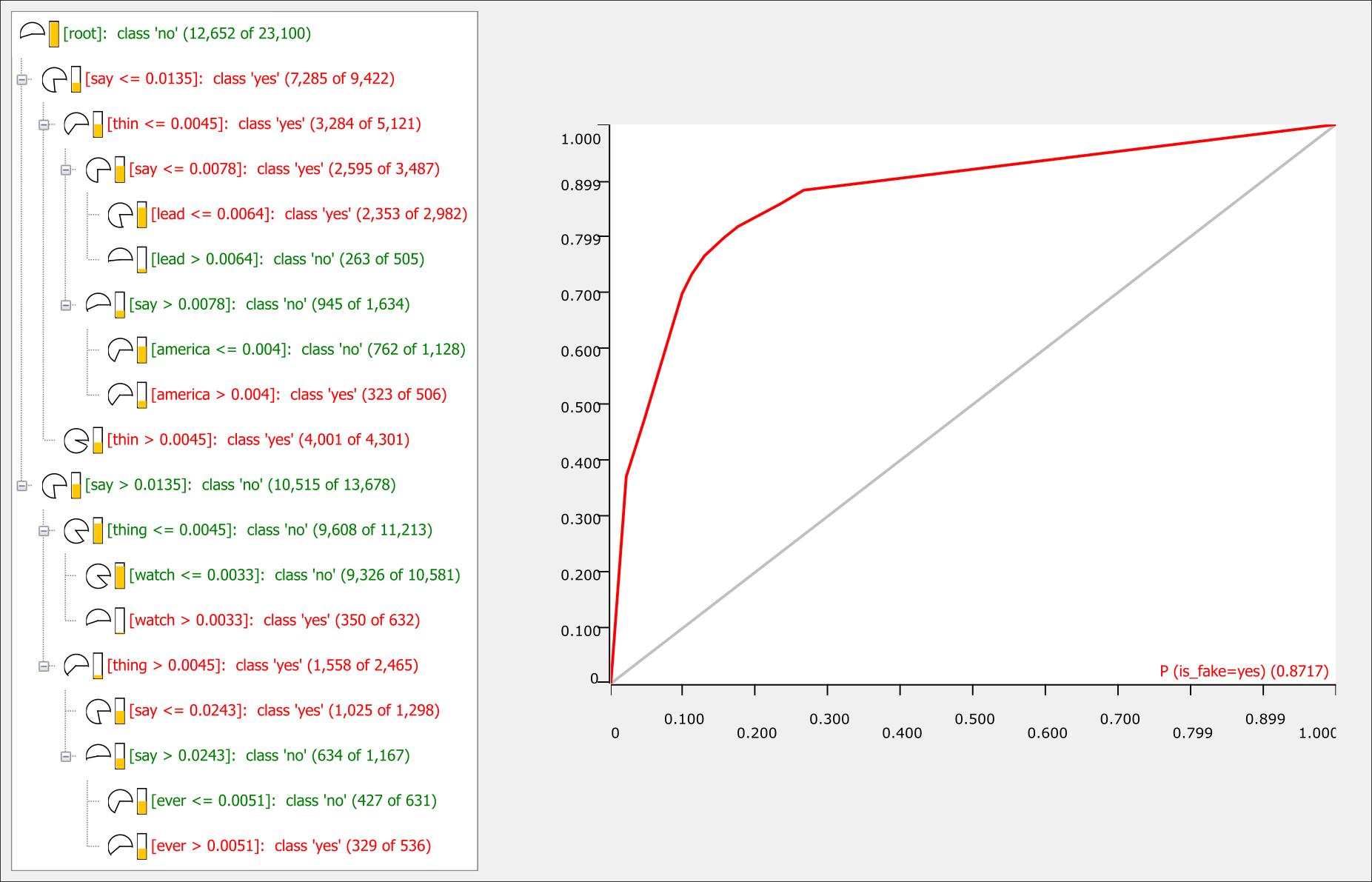
Single decision tree and ROC curve (click to view full size). In the tree layout, “yes” and “no” refer to whether an article is to be classified as fake news.

Some features in the tree layout are quite interesting to interpret. The first decision in classifying an article as “true” or “fake” is the lemmatized word “say”. For word frequencies at or below 0.0135, the tree tends towards a “fake” classification. This tells us that any derivative forms of this word (as in “said” or “says”) is much more likely to appear in the “true” articles than the “fake” ones. A quick analysis of the cleaned data before lemmatization confirms this: “said” appears almost 100000 times in the “true” news articles, but only about 25000 times in the “fake” ones (even though the latter subset is about 40% larger). Evidently, the “true” news from Reuters rely to a much higher degree on direct quotes than the “fake” news – which isn’t all that surprising. Furthermore, the appearance of “thin” as a discriminating feature can be explained by the widespread use of the phrase “thin skin” in the “fake” news; and likewise, articles that include videos often feature the word “watch” (typically in all-caps).

Regardless of the type of feature vector that is used (“binary”, word counts or frequencies), the accuracy of the decision tree is already around 80-83% on the validation set. Not bad for a such a simple model! The “kinks” in the ROC curve however reflect the fact that the classifications happen in a few rather discrete probability steps. So, let’s explore some more flexible models.

Random Forest

If one decision tree is good, then more decision trees are certainly better, right? The next logical step in our modeling is therefore to create either a gradient-boosted tree ensemble or a random forest model. Let’s test each option with a maximum tree depth of 10 nodes and see how the accuracies of these models evolve when we increase the number of trees. (Since tree ensembles are much more resource-consuming to train than random forests, we’ll also halve the number of trees in them compared to the random forests.)

Accuracy evolution of random forest (blue) and gradient-boosted tree ensemble (red) models with the number of trees. The arrow marks the accuracy of the previous decision tree. Note that the y axis starts at 70% for visual clarity.

Some differences in baseline accuracy for single-tree models exist due to random feature selecton in the random forests and lack of control over parameters such as the minimum number of records per node in the tree ensemble. Apart from that, increasing the number of trees in each model generally increases their accuracy; no big surprise here. Unfortunately, this comes at the cost of interpretability: For a single decision tree, explaining its structure is easy; for a bundle of 50 or 100 trees, it is not. So, even though we’ve been able to boost the modeled accuracy, we should look for some other strategy that affords us a better performance than the single decision tree while maintaining its explainability.

Logistic Regression

Departing from the use of decision trees altogether, we will next build a logistic regression model based on our feature vectors. Such a model is, in a sense, more “quantitatively” interpretable than the decision trees, since its parameters are directly comparable by their magnitude, and have significance estimates attached to them.

The latter point is also of high importance for the model building process itself, since we can eliminate highly insignificant parameters as judged by their p values to increase its robustness. We can set this up as an automated loop in KNIME, initializing the regression model with all 1100 parameters and successively eliminating all parameters with \(p > 0.05\) after each iteration. To improve convergence, we’ll also only discard 50 parameters at a time.

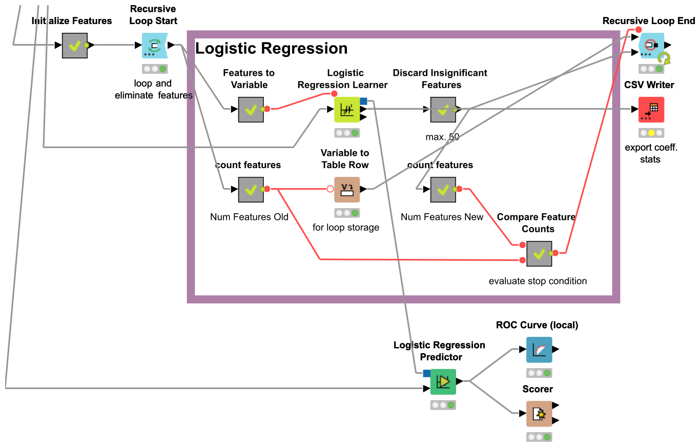
Simple, isn’t it?

After 21 iterations of this loop, we are left with 131 words that are deemed to be significant, yielding about 93% accuracy on the validation set. Of the selected features, 54 have positive coefficients (i.e., they indicate “fake” articles), and 77 have negative coefficients (indicating “true” articles). The five strongest “fake” words are gop, hill, watch, know and like; and on the “true” side, say, minister, trade, lead and representative.⁸

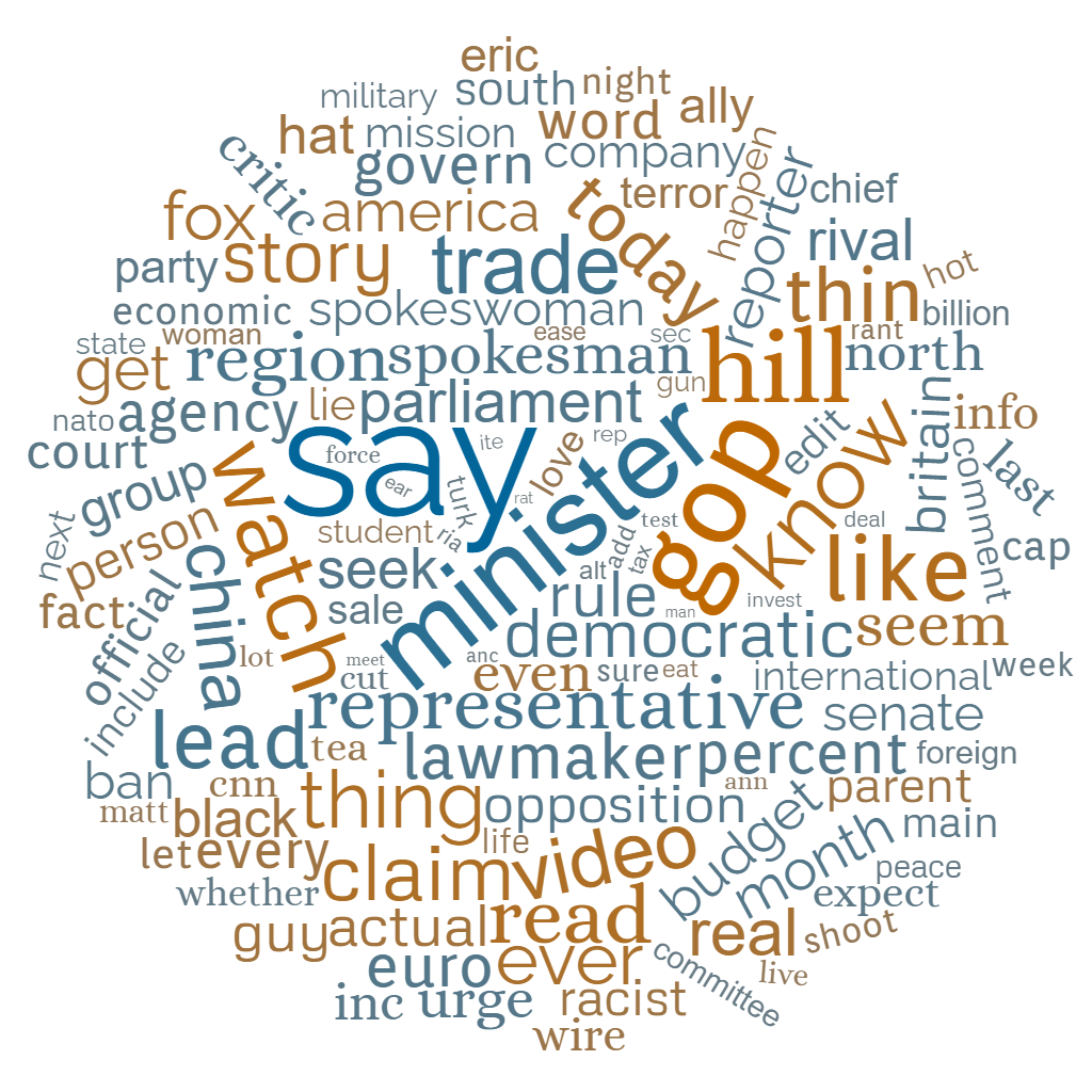
Blue words tend to classify as “true” articles, orange words as “fake” ones; word size and colour saturation indicate effect strength. Made using wordclouds.com.

With the numeric parameters from the logistic regression model, we can do another experiment: How does the accuracy of the model evolve if we only include a certain amount of the strongest parameters? In other words: What performance impact do we get from ignoring all signal words except for the top X% of positive and the negative parameters? This is easy to calculate by zeroing the input feature vectors for all excluded regressors and calculating the resulting performance statistics for the validation set.

Accuracy evolution of the logistic regression model with the amount of included features. For each data point, the given percentage of strongest parameters (positive and negative each) is retained, all other input features are zeroed.

Unsurprisingly, ignoring many of the “significant” words decreases the model performance – but not as strongly as we might expect. At the 5% mark, only the top two positive (say, minister) and top three negative (gop, hill, watch) features are included; yet the model still manages to predict three out of any four articles in the validation set correctly! Another point of interest are the accuracy “plateaus” around the 30% and 60% areas. Apparently, the combination of features that are selected at these percentages lead to essentially no net gain in model performance. Finding detailed explanations for this effect would however require a level of in-depth analysis that is beyond our current scope, so we’ll just accept this observation as a curiosity.

To be continued…